Super-zoomable graphs
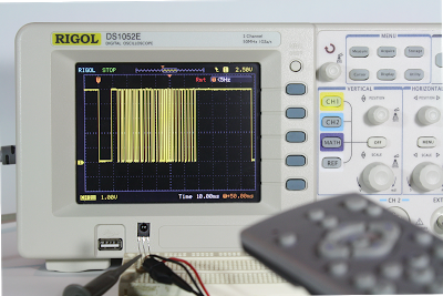
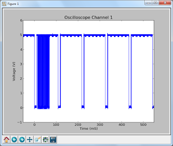
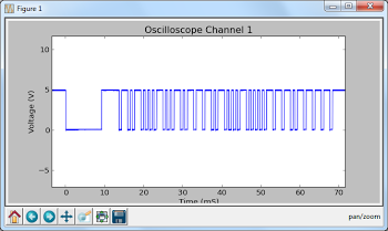
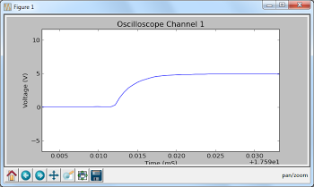
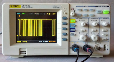
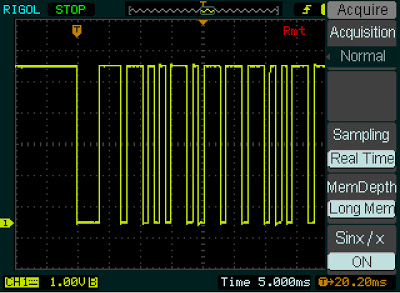
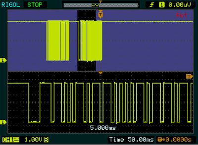
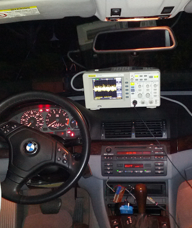
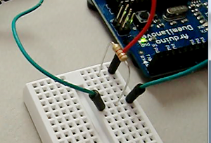
One of the nice features of the Rigol is "Long Memory" - instead of downloading the 600-point trace that appears on the screen, you can record and access a high-resolution trace of 1 million points. In this hack, I show how you can display this data with Python, giving you a picture that you can easily zoom into with the mouse.The following screenshot shows the data collected by hooking the oscilloscope up to an IR sensor. In the above picture, the sensor is the three-pin device below the screen. Since I've developed an IR library for Arduino, my examples focus on IR, but any sort of signal could be used. By enabling Long Memory, we can download not just the data on the screen, but 1 million data points, allowing us to zoom way, way in. The graph below shows what it sent when you press a button on the TV remote - the selected button transmits a code, followed by a periodic repeat signal as long as the button is held down.
To use this script, first enable Long Memory by going to Acquire: MemDepth. Next, set the trigger sweep to Single. Capture the desired waveform on the oscilloscope. Then run the Python script to upload the data to your computer, which will display a plot using matplotlib. To zoom, click the "+" icon at the bottom of the screen. This lets you pan back and forth through the data by holding down the left mouse button. You can zoom in and out by holding the right mouse button down and moving the mouse right or left. The magnifying glass icon lets you select a zoom rectangle with the mouse. You can zoom on your oscilloscope too, of course, but using a mouse and having labeled axes can be much more convenient.
A few things to notice about the code. The first few lines get the list of instruments connected to VISA and open the USB instrument (i.e. your oscilloscope). The timeout and chunk size need to be increased from the defaults to download the large amount of data without timeouts.
Next, ask_for_values gets various scale values from the oscilloscope so the axes can be labeled properly. By setting the mode to RAW we download the full dataset, not just what is visible on the screen. We get the raw data from channel 1 with :WAV:DATA? CHAN1. The first 10 bytes are a header and should be discarded. Next, the raw bytes are converted to numeric values with Mahto's formulas. Finally, matplotlib plots the data.
There are a couple "gotchas" with Long Memory. First, it only works reliably if you capture a single trace by setting the trigger sweep to "single". Second, downloading all this data over USB takes 10 seconds or so, which can be inconveniently slow.
Analyze an IR signal
Once we can download a signal from the oscilloscope, we can do more than just plot it - we can process and analyze it. In this hack, I decode the IR signal and print the corresponding hex value. Since it takes 10 seconds to download the signal, this isn't a practical way of using an IR remote for control. The point is to illustrate how you can perform logic analysis on the oscilloscope trace by using Python.
This code shows how the Python script can wait for the oscilloscope to be triggered and enter the STOP state. It also shows how you can use Python to initialize the oscilloscope to a desired configuration. The oscilloscope gets confused if you send too many commands at once, so I put a short delay between the commands.
Generate a spectrogram
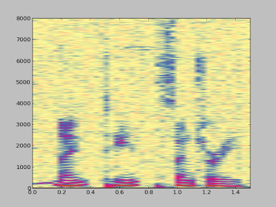
Another experiment I did was using Python libraries to generate a spectrogram of a signal recorded by the oscilloscope. I simply hooked a microphone to the oscilloscope, spoke a few words, and used the script below to analyze the signal. The spectrogram shows low frequencies at the bottom, high frequencies at the top, and time progresses left to right. This is basically a FFT swept through time.
Dump data to a .wav file
You might want to analyze the oscilloscope trace with other tools, such as Audacity. By dumping the oscilloscope data into a WAV file, it can easily be read into other software. Or you can play the data and hear how it sounds.
To use this script, enable Long Memory as described above, capture the signal, and run the script. A file channel1.wav will be created.
How to install the necessary libraries
Before connecting your oscilloscope to your Windows computer, there are several software packages you'll need.- I assume you have Python already installed - I'm using 2.7.3.
- Install NI-VISA Run-Time Engine 5.2. This is National Instruments Virtual Instrument Software Architecture, providing an interface to hardware test equipment.
- Install PyVISA, the Python interface to VISA.
- If you want to run the graphical programs, install Numpy and matplotlib.
VI_WARN_CONFIG_NLOADED errors. If you've already installed Ultrascope, you'll probably need to uninstall and reinstall NI_VISA.
If you're using Linux instead of Windows, see Mehta's article.
How to control and program the oscilloscope
Once the software is installed (below), connect the oscilloscope to the computer's USB port. Use the USB port on the back of the oscilloscope, not the flash drive port on the front panel.
Hopefully the code examples above are clear.
First, the Python program must get the list of connected instruments from pyVisa and open the USB instrument, which will have a name like USB0::0x1AB1::0x0588::DS1ED141904883. Once the oscilloscope connection is open, you can use scope.write() to send a command to the oscilloscope, scope.ask() to send a command and read a result string, and scope.ask_for_values() to send a command and read a float back from the oscilloscope.
When the oscilloscope is under computer control, the screen shows Rmt and the front panel is non-responsive. The "Force" button will restore local control. Software can release the oscilloscope by sending the corresponding ":KEY:FORCE" command.
Error handling in pyVisa is minimal. If you send a bad command, it will hang and eventually timeout with VisaIOError: VI_ERROR_TMO: Timeout expired before operation completed.
The API to the oscilloscope is specified in the DS1000D/E Programming Guide. If you do any Rigol hacking, you'll definitely want to read this. Make sure you use the right programming guide for your oscilloscope model - other models have slightly different commands that seem plausible, but they will timeout if you try them.
